Using Photoshop Histograms to Quantify Meteor Scatter Data

The usual way to quantify meteors is "one ping at a time."  I have described a method I use on 30m by watching pings on a local QRSS station.  It works well but is labor intensive and subject to false returns from airplanes...the local airport is between us.

Recently I've looked at two other ways to observe pings.  The web site LiveMeteors.com uses a well established technique which listens to the carrier signal from a Canadian TV station with a VHF receiving station in Washington DC.  I've had good results in using the audio piped into a PC sound card then to a waterfall spectrum analyzer,  Spectrum Lab.  Figure 1 is a typical recording.

Figure 1.  Typical Ping Recording for One Hour

The question arises immediately, "How does one count or assess all these pings?"  There's just too many to deal with, varying from specks to large events.  Photoshop to the rescue!  There's a similar problem in photography to evaluate at the tonal variation in a photographic image or parts of the image using a histogram of the luminosity.  Figure 2 is an example.  It is a graph of number of pixels in each exposure bin from 0 to 255, left to right, or pure black to pure white.  The significance is the mean or average grayness and the standard deviation which is a measure of the spread.  It seems to me that the mean best represents the intensity of the image but I have also examined the SD.  Here's how I did it.

Figure 2.  Luminosity Histogram

The pings were recorded in one hour chunks or "grabs".  For each grab I used the selection tool to make a rectangle around the significant extent of the pings and determined the mean within this frame.  Then to account for the background I moved the frame keeping the length and width the same to an area just below to measure the mean of the noise which I subtracted from the ping frame.  These values I assume are proportional to the intensity of the meteor shower for each hour.   Figure 3 shows the measurement frames for pings.  The frame was moved down to an area with no pings for the background.  Note that there is an extra line of pings above the main one and it is not relative to this discussion.

Figure 3.  Frame Selection for Pings Histogram

This procedure was applied to a 24 hour set of grabs made in one hour increments during a recent meteor shower and plotted to produce Figure 4.  The results shows the expected variation with maximum pings around Sunrise and minimum around Sunset.

Figure 4.  Results Obtained with Mean Luminosity Assessment of Pings per Hour

It is by far the quickest way to analyze pings I have tried.  Once the workflow was established I found it took only a few minutes to determine the histogram data for each one hour grab. Any method of quantifying meteors is relative since any measurement scheme counts pings only in a given field of view.  What I like about this method it that it takes into account pings of all size and strength right down to the background noise..

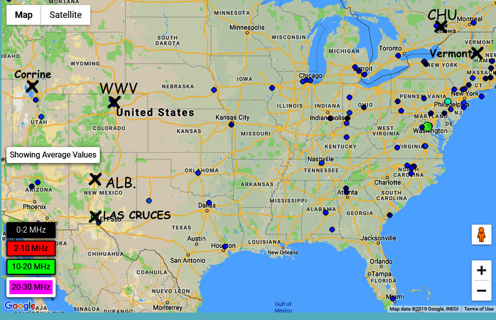
A second method utilizes receiving stations on the KIWI network which are tuned to strong stations such as WWV and CHU.  The audio is fed into my PC as described above and produces similar output. .  Both stations emit strong, omnidirectional  signals which are on the air 24/7 day in and day out.  The KIWI receiver network consists of dozens of KIWI-SDR receivers located around the World and controllable by the user via an Internet connection.   Figure 5 is a compilation of several combinations made back in late April as a first look at the feasibility of the method.  I have lately explored this in more detail with CHU on 14700 kHz using the KIWI receiver of W1NT in New Hampshire.  The antenna at W1NT is a 500 foot Beverage aimed northeast

Figure 5.  Feasibility Study of Using KIWI Receivers to Measure Pings from WWV and CHU

 and does a most excellent job of pulling in the weak QRSS stations running typically 250 mW signals on 30 thru 160m.  It should do even better on 14700 kHz and apparently does based on signals received so far.  Figure 6 shows a one hour grab using DL4YHF's Spectrum Lab software while Figure 6 shows greater detail using that of G3PLX's SBSpectrum software.  I can see the possibility of using the Mean Luminosity technique to isolate and record pings moving towards, upper, and away, lower, from the receiver.

Note the two horizontal lines at the center shown at higher resolution in Figure 6 where we see there is actually a third line in between.  This is the well known and commonly seen effect of backscatter

Figure 6.  Bragg Effect Backscatter by Ocean Waves

from surface waves on a body of water due to the Bragg Effect.  The moving waves cause a Doppler shift in which the intensity is made stronger by the regular spacing of the waves.    The fainter center line is the incident wave either reflected from land or possibly transmitted via ground wave.  I don't think this applies to meteors but there it is.

de bill w4hbk

Observing the 2019 Lyrids Meteor Shower using KIWI-SDR Receivers

I have previously described on this blog use of receivers on the KIWI-SDR network to make a QRSS grabber, http://pensacolasnapper.blogspot.com/2019/02/using-receivers-on-kiwi-sdr-network-s.html.
In this post I will describe the use of the KIWI's to record meteor pings using signals from WWV on 25 MHz and CHU on 14.7 MHz.  This is not QRSS but let me explain.

A group of the QRSS Knights in the UK have been able to record pings from their network of 10m QRSS signals.  It was my intention to join them during the recent Lyrids by using KIWI receivers around southern England where the QRSS transmitting stations are located but, alas, nothing was seen during two nights of observations.  The problem seems to have been with the lack of sufficiently strong pings as the UK stations that had previously seen good pings saw just one this year.

To see what the 2019 Lyrids looked like I decided to use signals from WWV and CHU as received by  KIWI receivers nearby on the day after the predicted peak.

For the WWV signal I chose two stations in New Mexico and one in Utah while for CHU a single station in New Hampshire was selected.  The choices were based on Signal to Noise Ratio data provided at the website operated by IS0KYB.  Here's a map of the stations involved:

Figure 1.  Location of Stations Used in This Experiment

The distances involved were:

WWV to Corrine, UT               373 mi/600 km
WWV to Albuquerque, NM     381 mi/625 km
WWV to Las Cruces, NM        577 mi/930 km
CHU   to Pittsford, VT             189 mi/304 km

Here's a grab showing typical pings for all stations:

Figure 2.  10 Minute Grab Showing Meteor Pings for All Stations

A comparison of pings shown in Figure 2 needs several comments.  Firstly, Las Cruces is  about  100 miles further away from WWV than Albuquerque yet has more and stronger pings.  This is simply because the former has a better antenna and lower local noise.  I also noted that a significant ping from Alb. usually coincided with a strong ping from Las Cruces. 

Secondly, Comparing Corrine, UT to Las Cruces the ping densities are similar when allowing for the different distances but those from Corrine are short and choppy while those from Las Cruces are much longer lasting.  This might be due to the path directions, i.e., East-West vs North-South but I have no reference for this.

Thirdly, the pings between CHU and Vermont are stronger and longer lasting.  The distance is much shorter that from those out West and as frequency goes lower pings last longer since higher electron densities are needed to support reflections at higher frequencies.

If you would like to read more about meteor pings and their signatures this is a good paper  on the subject by Peter Martinez, G3PLX.

In conclusion it appears there were plenty of rocks from the 2019 Lyrids stream but the strength and density must not have been sufficient to produce pings from the 100 to 200 milliwatt QRSS transmitters in the 10m UK network.

Appendex

Take a look at the study I did using a local QRSS station, KD5SSF, during the 2018 Geminids Meteor Shower which covered several days before and after the predicted peak.  It gives some idea of the statistical nature of showers for which in this case the predicted peak did not occur on December 23 but a day later.                                                                                                                                                                                                                                                                                                                                                                                                                                                                                                                                                                                                           

Using receivers on the KIWI SDR Network as remote grabbers

I had seen the KIWI SDR Network before but didn't realize just how good the receivers are.  After some experience I find that they are generally as good as a "real" receiver and by that I mean a standard HF transceiver such as my TS-440 or TS-480.  I feed the audio from a KIWI receiver into Spectrum Lab and end up with a grabber that looks and works  like the grabber with which I've had success over the years.

The above link will tell you how to find and log onto a given receiver which will open a screen like this one at EA2CQ, after selecting a few parameters in the control panel at lower right :

Figure 1.  KIWI SDR Display

Here is a more detailed view of the important parts:

Figure 2. Setup Details

First, enter the frequency of the center of the QRSS spectrum in the box at the upper left.  For the center frequency I use 100 Hz below the lower edge of the WSPR band which for 40m is 7039.9 kHz.  Then choose "cw" which will select a filter width, 400 Hz which is just right to cover 300 Hz of QRSS plus 100 Hz of WSPR.  I find being able to see some WSPR helpful when there might not be QRSS signals coming thru to have some idea if the band is open or maybe the KIWI station is using a poor antenna, etc.  Note at the top left the filter is shown centered on the frequency chosen.  You may have to use the mouse wheel to adjust the width of the spectrum.  Roll the wheel forward away from you to narrow the spectrum and backward toward ;you to make the spectrum wider.  Start with a narrow view to ensure the frequency is 100 Hz below the WSPR band edge.  You can then widen the spectrum to see what around and in fact go all the way to 0 to 30 MHz coverage without affecting the cw filter.

Then click on "Auto Scale" which usually makes a nice contrastl.  Finally, select a slower speed with "Slow Dev" which has 5 steps.  I find "Slow" or "1 Hz" works best.  These adjustments should give a nice image but you can play with the other controls for tweaking as desired.

At this point you should hear the audio from QRSS/WSPR around 500 Hz.  Now, direct this to your sound card and feed that into a waterfall/specturm analyzer such as Argo or Spectrum Lab you have a working grabber whose images can be uploaded to a web page just as you do with a receiver in your shack....except it is coming from a remote receiver.  Here is an example using a KIWI receiver I like in Tabov, Russia just west of Volgograd:

Figure 3.  Resulting QRSS Grabber Using Spectrum Lab

KIWI SDR is designed to produce audio for the speaker of your computer and it may be tricky to direct this to the sound card.  I use Windows 7 and had to enable Stereo Mix which is sometimes called "Recording What You Hear".  Right click on the speaker icon and select "Recording Devices" then right click on a blank area in the pane and ckeck "Show Disabled Devices" and "Show Disconnected Devices".  Click on Stereo Mix and enable it.  Then in the Audio Device selection of you spectrum analyzer (Argo or Spectrum) select Stereo Mix.

Now you should have a working grabber which I refer to as a "Hybrid Grabber."  This link will show you a map of all known receivers on the KIWI SDR Network.  Click on one and you're off and running.

I now have four images on my grabber.  The third one down is dedicated to KIWI SDR.  As you can see it looks just like the others that come from my Kenwood transceivers.

If you have problems my email is w4hbk@arrl.net

de bill w4hbk

* Select cw mode with receiver set for a cw note of 500 Hz....cw mode is actually in USB
** Offset based on a cw beat note of 500z

ps   here is a table of settings for each band:

QRSS Grabber Settings*

Band WSPR Low Edge QRSS Center Frequency Waterfall Offset**
80m 3570.0 kHz 3569.9kHz 3569.4 kHz
40m 7040.0 7039.9 7039.4
30m 10140.1 10140.0 10139.5
20m 14097.0 14096.9 14096.4
17m 18106.0 18105.9 18105.4
15m 21096.0 21095.9 21095.4
12m 24926.0 224925.9         24925.4
10m 28126.0 28125.9 28125.4

Quadrandids Meteor Shower Pings using QRSS Radio Technique

This is similar to the previous post about the Geminids Meteor Shower.  The difference is that I counted the number of 2 hour periods with a ping   In the previous study I noted if there was a ping or pings in a given 10 minute grab and then weighted it by a factor of 2 or 3 depending on how brightness and duration of pings.  I then totaled the pings counted is this way for 1 hour periods.  I think, or hope, this better represents the time history of the shower.

Experimental Technique

The stability of modern QRSS equipment is such that most signals on the Waterfall Display fall almost exactly on top on each other thanks to the design of the U3S QRSS transmitters available from QRP Labs.

This is considered a Bi-Static Radar.  The transmitting station is KD5SSF located in Pensacola, FL running about 200 milliwatts to an inverted V antenna.  The receiving station is W4HBK using an inverted V located 10 miles south in Gulf Breeze, FL.  I rotated the receiving antenna to minimize KD5SSF's

Figure 1 is a typical grab without evidence of any pings.   There are a few artifacts near the trace but they do not have the signature of a ping which is generally a fuzzy, displaced line parallel to the original trace.  Figure 2 is a grab taken during the shower to illustrate how I counted pings.

Figure 1.  Grab of KD5SSF without Pings

Figure 2.  Typical 10 Minute Grab with Pings

Note the marks at 2 minute intervals.  I noted if there was evidence of any ping in each interval and in this case there is for all 4 intervals so I assigned a "4" to this 10 minute period or grab.  The absence of signal from 10:40 to 10:42 is a cooling off period to avoid overheating of the U3S's final transistors.

There are problems with interference from other radio signals plus the echoes from aircraft activity at the Pensacola airport located between KD5SSF and myself, Figure 3.

Figure 3.  Airplane Interference

The actual counting was done by overlaying KD5SSF's signal on the screen of the display with Matte Finish Scotch Tape© and marking the 2 minute intervals.  Tape is perfectly clear and does not stick permanently.  Nevertheless, don't leave the tape on any longer than necessary as it might mar or damage the display..

Figure 4 is the a table of my counts.  The left column is the UTC hour interval and the right column is the counts for each 10 minute interval.  For example, look down the hour column to "04-05".  In the first 10 minute interval I counted 0 pings then 1, 1, 1, 0 and finally 3 in the 6th for a total of 6.

Figure 4.  Table of Counted Pings

Results and Discussion

Figure 5 is the histogram of UTC hour vs pings counted for each hour which illustrates the activity over a 24 hour period during this experiment.

Figure 5.  Results

Based on the hype I read before the shower I was expecting to see a sharp peak around 0300z but as you can see the pings were well below average at that time.  Instead, the peak is at about 0900z....what's up?

I should have read the "hype" a little more closely.  The Quadrantids is in a very narrow stream and should have produced a very high number of meteors around 0300z for observers in Europe and North Africa.  The radiant is near the Bootes constellation which at 0300z would have been just below the horizon at my QTH in Florida so that I would have missed the main peak.

There are two effects going on here.  First, the hourly meteor rate is falling off just as the peak comes into view.  Secondly, the radiant rises into view for me and like most meteor showers peaks between midnight and dawn when it was at its highest point in the sky around 0900z.  Figure 6 illustrates the effect.

Figure 6.  Effect of Radiant View on Meteor Stream

I don't know why there is a minor peak on the extreme left.  There must have been more structure to the stream than just a simple, sharply peaked bell shaped curve.

I reviewed the images and can see no blatant source of error.  In fact I probably under-counted pings due to rejecting frames with too many airplane reflections and QRM from the Cyprus radar that lasted from 0520 to 0720z

Conclusions

This is the second recording of pings using the somewhat subtle Doppler shifts occurring on a QRSS signal being observed and recorded using a waterfall display.  The fact that both follow the expected rise and fall of pings I believe validates this technique.  I see no reason why the ping rates I observe are not at least proportional to the true ping rates.  What's amazing to me is that this can be done with a simple transmitter running just 200 mW and modest antenna and receiving equipment.

The only drawback is that the two stations need to be at just the right distance so that the ground wave signal is not so strong as to overpower the receiver and thus reduce the sensitivity to the weaker Doppler signal.  It is also possible to rotate antennas and/or use opposing polarizations to obtain a "just right" signal level.

QRSS Signals as Indicators of Sporatic E

This is a quick compilation of observations taken during a Sporatic E opening recently on 10m.  I initially noted a fuzzy broadening on the signal of KD5SSF who is located 10 miles north of me and having seen it before thought that the only thing to cause it was reflections from a turbulent layer "up there".  On this occasion I had the presence of mind to check with the Sporatic E map provided online by G7IZU, which is compiled from reported QSOs on 10m and above.  Figure 1 is one of the maps showing the QSOs:

Figure 1.  G7IZU Sporatic E Map

The signal of KD5SSG observed at the same time is shown in Figure 2:

Figure 2.  KD5SSF Signal with Suspected Es Broadening

There is also a ionogram from the GIRO sounder 40 miles to the east of me which may also be showing ing reflections from an Es layer, Figure 3:

Figure 3.  Ionospheric Sounder from Eglin AFB 40 Miles to the East

Note in particular the reflections recorded along the bottom most trace...the others above it are roundtrip reflections which usually indicates a strong reflection.

My QRSS grabber was active on 10m at this time and the map shown at wsprnet.org looked like this"

Figure 4.  WSPR Spots Taken During the Es Opening

Putting it all together I think the broadening of KD5SSF's signal is caused by backscatter from an overhead Sporatic E cloud at a height of 100 km which is the average height of the E layer.  Also, the ionogram trace is showing the Es activity.  At least this is my guess at this time.

If you are close to a QRSS station and see a similar broadening it may be an indication that a Sporatic E layer is overhead.