Plotting Signal Strengths with Spectrum Lab

Spectrum Lab has a feature which allows one to bracket a signal on the waterfall display and watch its signal strength as a strip chart recording.  This feature is called "Watch List & Plot Window" and is found in the "View/Windows" menu at the top of the display.  Here's the set-up screen:

Set-up screen for SpectrumLab signal plotter.

It's a bit tedious to learn to use and involves a set of commands, functions and expressions reminiscent of BASIC which allow a signal on the waterfall display to be selected and plotted.  But the good news is that only a few instructions are necessary for making a simple strip chart recorder.  I use two expressions:  noise_n(f1,f2) which plots the band noise in the range between f1 and f2 which are two audio frequencies on the WF display and peak_a(f1,f2) which yields the peak signal between two frequencies.  Up to 6 signals may be selected and plotted at the same time.

The noise_n function divides the range between the two specified frequencies into 256 bins and averages the 1/4 lowest values to obtain the band noise.  The likelihood of including actual signals in this average is very low unless there is broadband interference present such as from RTTY or JT65.

The peak_a(f1,f2) expression brackets the signal of interest, divides it into 256 bins and selects the largest value to plot.  This makes a varying QRSS fskcw signal appear as a continuous line since the mark and space are always within the brackets.  Wolf thinks of everything.

OK, so why the interest in plotting signal strength?  One reason would be to watch for changes in your signal while doing some antenna comparisons, for example.  Another and the one in which I'm interested is to study QSB.  There are three causes of QSB:  multipath interference, Faraday rotation and ionospheric focusing.  In multipath the signal is reflected from two or more layers and arrives at the rx antenna to interfere destructively and constructively.  In Faraday rotation the polarization of a linear transmitted wave rotates as it passes thru the Earth's magnetic field and arrives at the polarized rx antenna at a state other than of the tx antenna, ie a vertically polarized transmitted wave can arrive at the rx as another polarization, including eliptical.  Focusing is cause by the shape of the ionosphere which can vary from convex to concave.

Scientist and engineers who study propagation have utilized simultaneous recordings of the vertical and horizontal vectors to detect the Faraday effect and the qualitative nature of the overall variations to separate the three effects.  It ain't easy and requires sophisticated computing capability and understanding of propagation, definitely a job for professionals.  However, that doesn't keep we amateurs from having fun with the subject, making our own observations and attempting to guess which effects are occurring.

My favorite reference on QSB is the dissertation of Dr. Yau at the University of Adelaide who studied the effect on OTHR signals in the 6 to 10 MHz range.  There's a good discussion of hf propagation there plus a details of the receiving apparatus and computational techniques.  Imagine getting a PhD in QSB!

Here's an example of QSB recordings I've made on some 30m signals:

Example of strip chart recording

The Red trace is the band noise, Yellow is KD4PBJ near Chattanooga, TN and Green is AK4T near Atlanta, GA.  

de w4hbk

Dopplergram Catches a Solar Flare

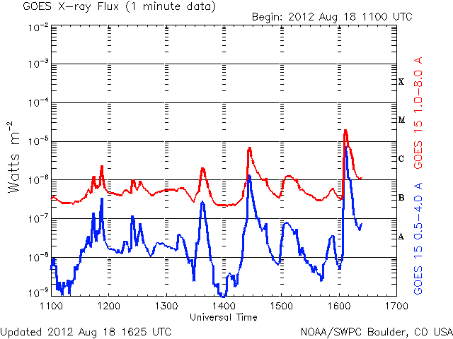
Yesterday I took a day off from grabbing to try my new Dopplergram on the WWV 10 MHz signal.  As luck would have it an M-class Solar Flare occurred during the recording:

Figure 1.  Solar Flare of 18AUG12 as seen on Dopplergram

Figure 2.  Solar Flare of 18AUG12 as seen on 10 minute grabber

Figure 3.  GOES X-ray flux

An M-class flare commenced just before 1610z.  The increasing frequency means the path length was decreasing as the reflecting layer moved downward

This is the cleanest data I've recorded of a flare and justifies a calculation of Ionospheric motion from the observed Doppler shift.  I assumed a simple triangle relationship of the radio path (Earth's curvature ignored) and obtained distance parameters via the Internet and the take-off angle of the signal from W6EL's propagation program.  The calculations are as follows:

Figure 4.  Calculations of vertical velocity of Ionosphere in response to Solar Flare of 18AUG12

The estimated vertical velocity of the reflecting layer was ~ 250 km/hr for a 1 Hz shift or 750 km/hr (466 mph) for the maximum 3 Hz shift as seen in Figure 2.

If we assume the average speed was 104 m/s (corresponding to an average Doppler shift of 1.5 Hz) then the distance moved by the Ionosphere over a period of 45 seconds was  4.7 km which is small compared to the starting distance, h, of 217 km.  Thus h can be assumed constant.

Bottom line:  the Ionosphere moved vertically downward in response to the stimulus of the Solar Flare at an average speed of 500 km/hr (310 mph).

There is a nice discussion of the Doppler effect at Wikipedia and you can check my math since I've been retired for almost 20 years now and seldom use calculus any more.

CME Effect on 40m QRSS Signal

This post is to document the effect of a Coronal Mass Ejection (CME) on a QRSS signal propagating between New Mexico (WA5DJJ) and Florida (W4HBK).  The CME occurred on July 12 and was described in my last post.

Figure 1 shows the observed effect.  DJJ transmits a fsk cw signal referenced to a Rubidium frequency standard which at this time scale produces two parallel lines corresponding to the fsk mark and space.  The Master Oscillator of my TS-440 is temperature controlled, thus the observed frequency changes are due to Doppler shifts caused by motion of the ionosphere.   As luck would have it, Dave's signal came on just before the start of the disturbance while the QRM ceased at the same time.

Figure 1.  Frequency shift of WA5DJJ signal during geomagnetic disturbance

Note these features:

1.  Start time is about 0345z
2.  As the event progressed four separate layers developed as the frequency shifted downward followed by a reversal with a decaying sine wave pattern.
3.  The apparent speed of the wave was very slow with a period or 1 to 2 hours.

Figure 2 is a corresponding magnetometer recording from Anchorage, AK which indicates time history of the geomagnetic disturbance.

Figure 2.  Geomagnetic disturbance recorded at Reeve Engineering Labs in Anchorage, AK

This leaves little doubt that the observed effect on the QRSS signal was caused by the disturbance.  However, this was not the initial arrival of the CME.  As shown in Figure 3 that actually occurred the day before at 1700z.

Figure 3.  CME history recorded by ACE spacecraft (~ 1 hr before before seen at Earth)

Our observation was related to the minor hump occurring at about 0300z.  I had made an effort to be watching for the arrival as predicted at solarham.com but, again as luck would have it, the presence of lightning forced me to secure my station at that time.

Here's how I visualize the storm as depicted in Figure 1.  After the particles slammed into Earth around the Auroral Zone an ionospheric wave spread out at a surprisingly slow speed.  This wave is indicated by the exponentially decaying sine nature of the frequency variations.  The splitting of the frequency into 4 components is also surprising and could imply either a stacked vertical layering or possibly skip points spread out horizontally...but why 4?  In conclusion, I find both the layering and the slow speed with which the disturbance spread to be remarkable.

de w4hbk

Measurement of 30m Noise Background at W4HBK

In my last post I described a method I use to disengage the AGC of my TS-440 so that accurate measurements of signal levels can be made.  Last Winter I tried to measure the background noise on my receiver but found that AGC compression was a major problem.  Now that I have that ironed out I've tried again to measure the background noise, this time with success.

My system consists of an Inverted V antenna into a Kenwood TS-440 receiver whose audio output goes to a computer sound card and then the Spectrum Lab software.  All signal levels to which I refer are as measured on the SL display.  I define background noise as the signal level of the noise above the noise floor of my receiver which is determined by replacing the antenna with a 50 Ohm resistor.

I used a little know feature of Spectrum Lab called "Watch Window"   to record my data. WW allows you to select a specific part of the spectrum to be recorded as a strip chart, e.g., amplitude vs time.  I described this in a previous post called "New Toy" back in March.  Several expressions are available to measure both signals and noise.  The noise expression is,

     noise(freq1, freq2)

which measures the noise level between f1 and f2 and eliminates the effect of discreet signals using the following scheme:
   1.  an array of amplitudes from the last FFT calculation is sorted into order of increasing amplitude.
   2.  The amplitude of the lower quartile value is then returned as an estimate of the mean noise level. 

With the frequency range set to cover 10140.0 to 10140.1 and numerous QRSS signals present it ignores them and measures just the noise....like magic  You can read about this in more detail in the SL help file.  The only problem I've had is with strong RTTY and JT65 signals which cover the entire QRSS spectrum but this is rare and easily recognized..

I recorded the noise background for a 24 hour period so see how it varied with time of day.  The results are shown in Figure 1.  The spikiness is due to static crashes plus occasional clicks and pops from electrical equipment.  I can hear nothing that sounds like power line noise or crt emission, etc....just the steady crunch of sferics.  Thunderstorm activity was actually mild during the measurement period with just a few small storms no closer than 25 miles, indicating to me that the sferics were propagating in from afar.

Figure 1.  Noise vs Time of Day Measured @ W4HBK

The time of maximum noise was just around sunset at about 35 to 40 dB above the NF.  Minimum noise occurred around noon at 20 to 25 dB above the NF.

For comparison I obtained the noise estimate from VOCAP, Figure 2.  The trend for time of day is close but I measured a max to min range about twice as large as VOCAP, 15 dB vs 7 dB, respectively.  My measurement is for a particular day whereas the VOCAP estimates are based on extensive observations used to determine averages.

Figure2.  VOCAP Prediction of Noise @ Receiver

I plan to repeat the measurement several times to better characterize this time of year and then do the same for other seasons.  Can't wait for a cold Winter night to see how low we can go.

de w4hbk

FollowUp on Using WSPR Data

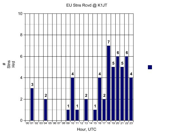
A few hours ago I checked the 20m WSPR data for the EU to NJ path during the past 24 hrs.....what a difference from the past weekend!  See for yourself:

Figure 1.  EU stations heard @ K1JT on May 21

Figure 2.  EU stations heard @ K1JT on May 24

Apparently condx were terrible over the weekend while my grabber was on 20.  The only dx station I heard was G6AVK and just for a few hours around 2300z.  If we had been on the past 24 hours I should have heard EU longer and probably louder.

The reason I'm interested in all this is that I've been thinking of moving my grabber to one of the higher bands during my local daylight  (1300z to 2300z) since that is usually when the dx comes thru to Florida.  But not being one to beat a dead horse I want to have some assurance of success.  My plan is to keep and eye on WSPR data as a guide to which bands and times to be QRV, particularly as a supplement to standard propagation predictions.

de w4hbk

P29ZL

The signal of P29ZL caught my attention soon after it's appearance on my grabber last month for two reasons.  First, it appears almost every night for about 5 hours, very strong and easy to copy.  But equally interesting is the extreme multipath/Doppler effect which is always present for at least part of the time.  Tim's mept, from the WA5DJJ Labs,  runs 250 mW to an inverted V hung in a 25 foot banana tree.  Figure 1 is a 5 hour grab from a few nights ago and is typical of what I see every night:  note in particular the considerable fuzziness of the signal between 1000 to 1100z.  Figure 2 is from the 10 minute grabber and shows the effect in more detail.  Other signals from out that way, most notably VK6JY show just a bit of broadening but nothing like that from P29ZL.

Figure 1 - P29ZL on the W4HBK 5 hr grabber, 12Apr11, 30m 

Here is my understanding of the multipath/Doppler effect.  As the signal passes through the ionosphere it may be partially refracted back towards Earth but a part may continue on to find another refracting region for a second signal, an so on.  At the same time multiple hops can occur with the results that a number of signals can arrive at the receiving antenna.  But for a Doppler shift to occur these various regions must be moving relative to one another.  Without this relative motion the signals arriving from the various paths would be at the same frequency but differing in phase to cause fading due to interference.  Other phenomena such as ionospheric irregularities and turbulence can also contribute a continuous broadening....visualize an eddy where some of the electrons are moving towards and some away from the path of propagation.  I've noticed that most writers of the scholarly articles end up stating how complex is the ionosphere....as the kid next door says to me sometimes. "Well, Duhhh!"

Usually the M/D effect is relatively simple with just 2 noticeable frequencies and I see this almost every day on one signal or another as the band is changing around sunrise/sunset.  What makes the fuzz on P29ZL's signal unique is that it's a daily occurrence with a near-continuous broadening, usually towards a higher frequency which would indicate the path length is decreasing.  Sometimes one or two distinct frequencies appear out of the continuum.

Enough for now about this most interesting signal but I will be keeping an eye on things and doing a bit more reading.

de w4hbk